A basic macroeconomic model of energy depletion in the presence of an alternative energy source

Written by Sam Wheldon-Bayes

Category: Ecological Economics; Long Read
Date: Monday 6 May 2019

Introduction – why system dynamics

System dynamics modelling has grown alongside the development of modern computing, starting with Forrester’s World Dynamics (1971). The purpose of system dynamics modelling is to form an explicit picture of a system that allows a researcher to understand relationships between the elements in that system, particularly feedback loops (Wolstenholme, 2003), as “it is often easier to act on system relationships than on system elements” (Meadows, 1982). In this way, the complexities of the real world can be reduced, with the ability to focus on leverage points when looking at changing a system (Meadows, 1999), or tipping points and limits when seeking to understand it (Meadows, 1972). A pluralist approach, in which diverse ways of understanding a system are compared, may prove particularly fruitful by overcoming effects generated solely by idiosyncrasies of model specification.

Research question

I aim to use a simple representation of an energy-dependent capitalist economy to model the responses of that system to gradual depletion of its primary energy resource, and transition to reliance on a more expensive alternative energy source. I use a pension fund as a representation of a capitalist system. It has savings inflows, consumption out of wealth and reinvested profits, which are all features of capitalist economies relevant to this exercise. I seek to understand the implications of this rise in energy prices in terms of the economic sustainability of the system. I test various specifications of energy price, alternative economic parameters such as wages, and the effects of an aging population.

Assumptions and model construction

Distribution

Workers (L) earn fixed wages (w) and pay a fixed fraction (s) of these into a pension fund. This pension fund represents the wealth (K), or capital stock, of the system and makes fixed payments ( $w_G$ ) to pensioners (G). All savings are assumed to be invested, meaning that there is no scope for effective demand in the system, but energy costs can constraint production, in which case labour and capital are both used at a rate $u$ . Profit ( $\pi$ ) is reinvested, and depends on price of energy, ( $p_E$ ), energy used (E) and wage costs ( $uwL$ ). The capital stock depreciates by a fixed percentage (d) each year. I assume a unit price index throughout, so the economy is effectively a barter economy with no role for money.

Production

I assume production ( $Q_S$ ) uses labour, capital and energy. Cobb-Douglas production functions allow substitution between factors of production, which is argued to violate fundamental laws of thermodynamics if energy is included (Dafermos et al, 2017). Leontief production functions specify fixed, technologically determined ratios between factors, which is unsuitable for a model such as this one in which accumulation is a key driver of system behaviour. To preserve substitution between labour and capital while treating energy as a fixed factor of production, I use a hybrid of a Cobb-Douglas production function and a Leontief production function (see appendix for discussion):

$Q_S={\rm min}\left\{ \alpha_{LK} (LK)^{\frac{1}{2}} , \alpha_E E \right\}$

Energy

I assume that the price of energy depends on remaining reserves of hydrocarbon energy (H), a fixed minimum that represents extraction cost ( $k_1$ ), a ratio that represents the price of the alternative energy source relative to base price ( $k_2$ ) and a coefficient of sensitivity ( $k_3$ ), taking the form

$p_e(H) = \left\{\begin{array}{rl}k_1\left(1+(k_2-1)e^{-\left(\frac{H}{k_3}\right)^2} \right),&H>0\\k_1k_2,&H\leq0\end{array}\right.$

I assume that since represents the price of supplying alternative energy to the entire system, it is reasonable to set this higher than currently used alternative energy sources.

Population

Workers enter the economy at a fixed rate ( $r_1$ ), with a one-time training cost (T) removed from the capital stock. They then retire at a fixed rate ( $r_2$ ), and pensioners die at a fixed rate ( $r_3$ ). Apart from the scenarios where a reduced death rate is investigation, these rates are set to produce a stable population of 700 workers and 300 pensioners.

Simulations

Varying energy price

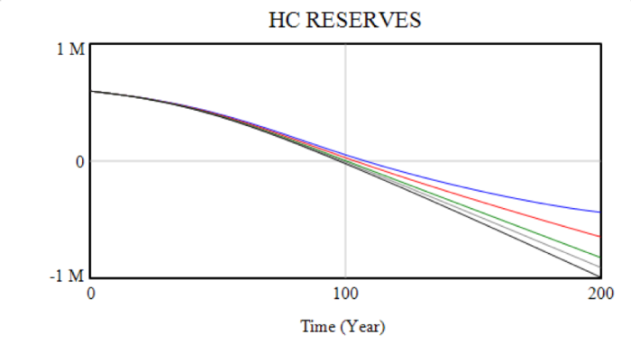
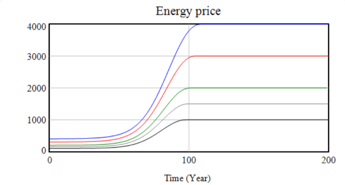
Graphs showing the behaviour of the system varying the base energy price between $100 and $400, with an alternative price ratio of 10. The system displays qualitatively different behaviour at different prices, with potential for system crashes, continuous growth or decline-and-stabilisation. The first two graphs show the depletion of hydrocarbon reserves and energy prices.

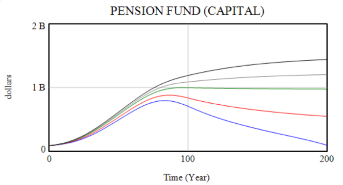
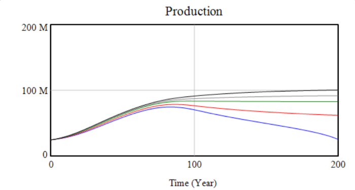
The next two graphs show the impact these changes have on wealth and production. Depending on the base energy price, the system either slowly crashes or finds stability. The depreciation term prevents unlimited accumulation.

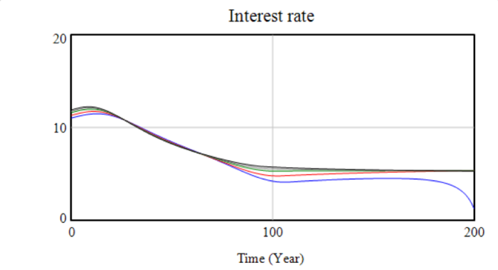
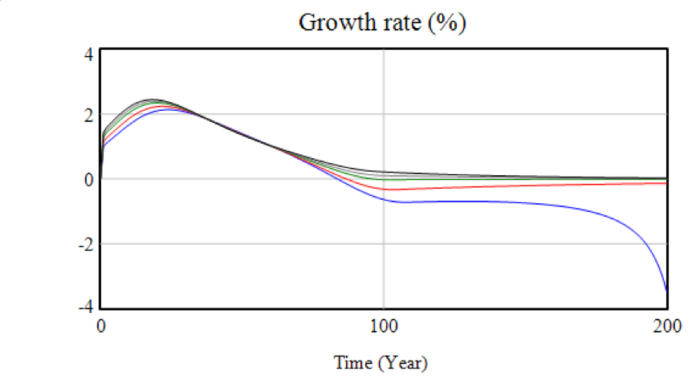
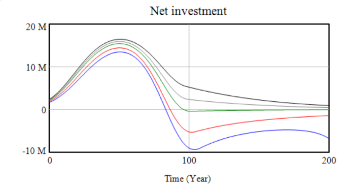
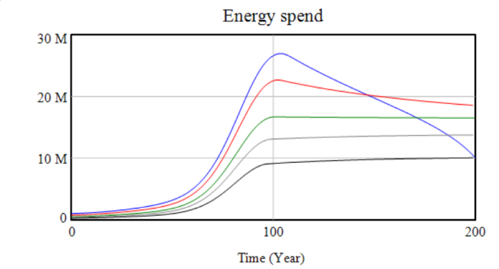
The last four graphs show various indicators derived from the variables – interest rate and growth (both of which are within realistic ranges) as well as energy spend and net investment. The growth rate variable shows the accelerating decline of the system once productive capacity begins to be lost.

Varying effective savings rate

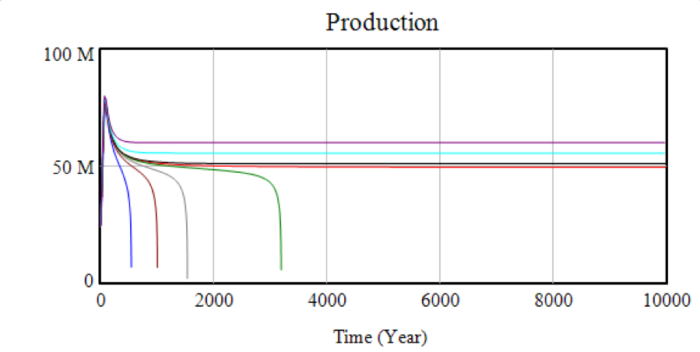
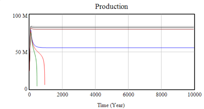
The system conforms to so-called “classical” behaviour in that growth is savings-driven. Increasing the contribution rate of workers or decreasing the wage (which increases the overall propensity to save) increases income. To illustrate, the case of a base energy price of 300 with an alternative price ratio of 10 was selected from the initial scenarios for displaying interesting long-run behaviour – negative growth but at a declining rate. Initially set at 20k, the wage was varied between 18k and 21k and the maximum time increased to 10,000 to capture long-run behaviour. The first two graphs show capital stock and production – slight changes in the wage determine long-term stability and have a huge effect on the time taken to collapse or the equilibrium level obtained.

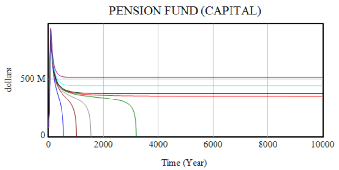
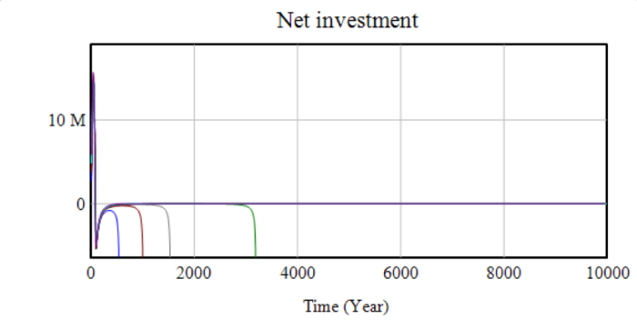
The key variable in determining the long-run stability of the system is net investment (NI).

$NI = \pi+ s(uwL) - \frac{d}{100}K - w_G G - (r_1L)T$

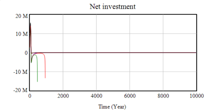
If initial net investment is below zero, the system loses capital and rapidly crashes as the reduced capital stock reduces production. If initial net investment is above zero, the system will grow rapidly until it is constrained by energy price rises or depreciation, which limits growth as capital (alone) displays decreasing returns to scale. If energy price rises cause net investment to become negative, system behaviour is highly parameter-sensitive. The next graph shows net investment, initially positive in each scenario – marking the “accumulation phase” – until this is wiped out by energy price increases. As the energy price maxes out at the point hydrocarbon reserves are depleted and the energy source is switched, about 100 years in, the economy begins to stabilise, but drops off in some scenarios.

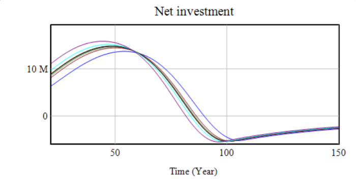
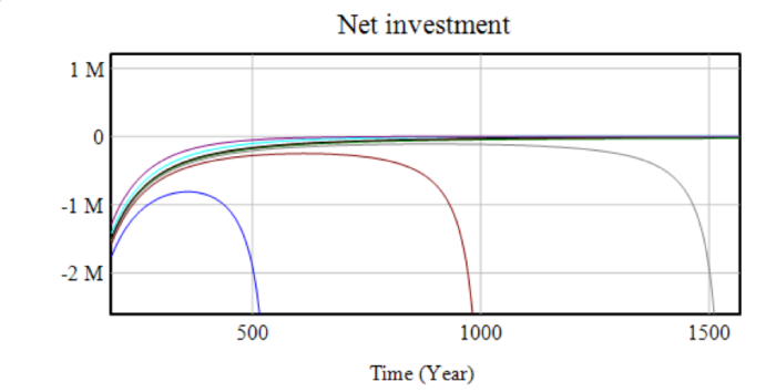
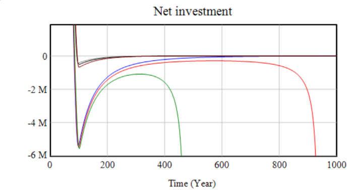
The next two graphs show selected ranges of net investment in more detail. The first graph shows the similarity of the different scenarios in the initial phase. The second shows that in the higher-wage scenarios, net investment begins to tend towards zero, but does so insufficiently quickly, and production declines too far to sustain. This behaviour is due to the decreasing returns to each individual factor – each unit of capital removed by negative net investment will be more productive than the previous unit removed. The critical wage (given the other parameters) in this scenario appears to be about $19,500, though even with a wage of $20,000, the model takes around 1000 years to fully crash – far longer than the stable structure of any model could be expected to hold.

Aging population

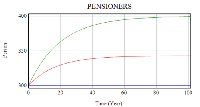
Initially, the birth rate, retirement rate and death rate were set such that both population and demographics remained constant, with a worker population of 700, a pensioner population of 300 and 20 births, death and retirements in each period. Decreasing the death rate from 8/120 to 7/120 and 6/120 produced equilibrium pensioner populations of 300, 343 and 400 respectively. With a wage of $19,000, and a base energy price of either $200 or $300, the long-term stability of the system was affected by the demographic shift.

In the lower-price case, the increase in pensioner population only had a small effect on the equilibrium level of production. In the higher price case, the effect on net investment was just enough that the system did not reach stability. The first graph shows the changing population (note that the grey, black and brown lines are hidden behind the blue, red and green lines, respectively). Subsequent graphs display wealth, production, net investment and a highlight of the critical portion of net investment.

Extensions, criticisms and comments

System dynamics approach

The system dynamics approach has been criticised from many angles (Featherston and Doolan, 2012). Forrester (2007) takes issue with the size and complexity of many models, which leaves them difficult to understand. Other critics, such as Solow (1972) and Simon (1981), believe that system dynamics models typically do not predict reality well, or take issue with the realism of assumptions used. These criticisms are slightly misplaced if the main aim is to understand dynamics of system behaviour, not to mimic or predict it.

System dynamics is essentially a reductionist programme (Keys, 1990), which seeks to reduce complex phenomena into the minimum number of hard rules which can describe the system. Social reality is general considered to be “open” (Lawson, 2006), so this leaves the system dynamics programme unable to realistically describe the nature of social change – which, in a sense, is about the shifting structure of a model. System dynamics is appropriate for describing simple mechanistic responses with complex interactions, not complex responses themselves.

Investment, demand and inflation

As mentioned above, in this system there is no role for effective demand, as all savings are assumed to be invested. A useful extension might be to drop the assumption that savings are equal to investment and allow some level of demand-determination (Keynes, 1936). Practically, this might be best achieved through a Kaleckian model (Kalecki, 1971; Rowthorn, 1982), extended along the lines of Bhaduri and Marglin (1990), who suggest an investment function dependent on expected profits, though Kaleckian models are generally difficult to reconcile with supply-side effects. Technological development over time might also be a useful area of study, as well as wages that vary with production.

Energy supply and demand

The assumption that the alternative price of energy should cost quite so much relative to base extraction cost may be hard to sustain. In addition, the range of reserves over which price increases might feasibly be much larger. Presently energy price increases are confined to between about 50 and 100 years, when energy is depleted. Investment into exploration for hydrocarbons could also be explored. To study energy depletion, the stock of undiscovered resources would need to be specified, so this might not change the fundamental long-run dynamics of the system but could introduce interesting non-linearities. Parameters such as the price of the alternative, or the energy efficiency of the economy, could be allowed to vary over time.

Classical political economy

Interesting classical political economy generally separated the factors of production into land, labour and capital (Smith, 1776; Ricardo, 1817). This reflected the reality of economies at the time, which were heavily agriculture-dependent, hence land was a critical limiting factor to production. This method of study of a may be useful for understanding stable systems. As Sraffa (1960) notes: “in a system in which, day after day, production continued unchanged in [scale and factor proportions] the marginal product of a factor would not merely be hard to find – it just would not be there to be found”.

Policy and conclusions

The restrictive assumptions of the model with regards to demand, and lack of realism in various parameters chosen means this model should not be used to draw concrete policy conclusions. Nonetheless it can paint an interesting picture of the sustainability of superannuation-type pension schemes within the context of energy depletion. Any attempt to use the framework this model provides to guide policy should attempt to maintain realistic assumptions about demand – given that we are dealing with a declining economy – and find realistic values for parameters. Even then, it should be treated only as an explanation of possible behaviour. Like all models it is, in the words of Meadows et al (1972), “imperfect, oversimplified, and unfinished.”

References

Bhaduri, A. and Marglin, S. 1990. Unemployment and the real wage: the economic basis for contesting political ideologies. Cambridge Journal of Economics. 14,pp.375–393.

Dafermos, Y., Nikolaidi, M. and Galanis, G. 2017. A stock-flow-fund ecological macroeconomic model. Ecological Economics.131,pp.191–207.

Featherston, C. and Doolan, M. 2012. The 30th International Conference of the System Dynamics Society In: A Critical Review of the Criticisms of System Dynamics. St Gallen.

Forrester, J.W. 1971. World Dynamics. Wright-Allen Press.

Forrester, J.W. 2007. System dynamics—the next fifty years. System Dynamics Review. 23(2/3),pp.359–370.

Kalecki, M. 1971. Class Struggle And The Distribution Of National Income. Kyklos. 24(1),pp.1–9.

Keynes, J.M. 1936. The general theory of employment interest and money. London: Macmillan.

Keys, P. 1990. System dynamics as a systems-based problem-solving methodology. Systems Practice. 3(5),pp.479–493.

Lawson, T. 2006. Economics and reality. London: Routledge.

Meadows, D.H. 1972. The Limits to Growth. New York: Universe Books.

Meadows, D.H. 1982. Whole earth models and systems. The Coevolution Quarterly.,pp.98–108.

Meadows, D.H. 1999. Leverage points: places to intervene in a system. Hartland Four Corners, VT: Sustainability Institute.

Ricardo, D. 1817. On the principles of political economy, and taxation. London: John Murray.

Rowthorn, R. 1982. Demand, real wages and growth. Studi Economici. 19,pp.3–54.

Simon, J.L. 1981. The Ultimate Resource. Princeton, NJ: Princeton Univ. Press.

Smith, A. 1776. An enquiry into the nature and causes of the wealth of nations. London: W. Strahan and T. Cadell.

Solow, R.M. 1972. Unknown. Newsweek.,p.103.

Sraffa, P. 1960. Production of commodities by means of commodities: prelude to a critique of economic theory. Cambridge, UK: Cambridge University Press.

Wolstenholme, E.F. 2003. Towards the definition and use of a core set of archetypal structures in system dynamics. System Dynamics Review. 19(1),pp.7–26.

Appendix

Assumptions and model construction

Production

Cobb-Douglas production functions take the general form $Q_S = k\Pi_{i=1}^n F_i^{\alpha_i}$ , where $F_i$ are the factors of production, $\alpha_i$ their respective coefficients and $k$ is a constant representing productivity; factors of production are infinitely substitutable, though with diminishing returns to substitution. Note that if $\sum_{i=1}^n \alpha_i = 1$ , the system displays constant returns to scale. Leontief production functions assume technologically determined ratios of production – so no substitutability of factors – and take the form $Q_S = {\rm min} \left\{ \alpha_1 F_1, , \alpha_n F_n \right\}$ .

Energy

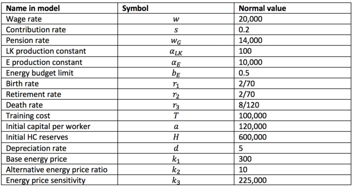
In determining energy demand, I assume firms are willing to spend no more on energy than a fixed proportion of their production from the previous period ( $b_E$ ). This proportion is set at 0.5, and never exceeded in the scenarios I run. Extensions of the model would better develop this very crude approach.

Typical values of parameters

Unless otherwise stated, model parameters are as follows

Reading the model

Stocks are coloured blue, parameters pink, auxiliary variables orange, and auxiliary variables that are of interest themselves are coloured green. Indicators that are not used in the model but helpful for understanding system behaviour are in grey.

Some portions of the model – specifically dealing with demand and energy budgeting – are not utilised under the current specification. As these are potentially interesting extensions to the model, the framework to incorporate them is retained.

Introduction – why system dynamics

Research question

Assumptions and model construction

Distribution

Production

Energy

Population

Simulations

Varying energy price

Varying effective savings rate

Aging population

Extensions, criticisms and comments

System dynamics approach

Investment, demand and inflation

Energy supply and demand

Classical political economy

Policy and conclusions

References

Appendix

Assumptions and model construction

Production

Energy

Typical values of parameters

Reading the model

Author

Sam Wheldon-Bayes